Steps 1-6
- Load the R packages we will use.
- Read the data in the files,
drug_cos.csv,health_cos.csvin to R and assign to the variablesdrug_cosandhealth_cos, respectively
drug_cos  <- read_csv("https://estanny.com/static/week6/drug_cos.csv")
health_cos  <- read_csv("https://estanny.com/static/week6/health_cos.csv")
- Use glimpse to get a glimpse of the data
drug_cos %>% glimpse()
Rows: 104
Columns: 9
$ ticker       <chr> "ZTS", "ZTS", "ZTS", "ZTS", "ZTS", "ZTS", "Z...
$ name         <chr> "Zoetis Inc", "Zoetis Inc", "Zoetis Inc", "Z...
$ location     <chr> "New Jersey; U.S.A", "New Jersey; U.S.A", "N...
$ ebitdamargin <dbl> 0.149, 0.217, 0.222, 0.238, 0.182, 0.335, 0....
$ grossmargin  <dbl> 0.610, 0.640, 0.634, 0.641, 0.635, 0.659, 0....
$ netmargin    <dbl> 0.058, 0.101, 0.111, 0.122, 0.071, 0.168, 0....
$ ros          <dbl> 0.101, 0.171, 0.176, 0.195, 0.140, 0.286, 0....
$ roe          <dbl> 0.069, 0.113, 0.612, 0.465, 0.285, 0.587, 0....
$ year         <dbl> 2011, 2012, 2013, 2014, 2015, 2016, 2017, 20...
health_cos %>% glimpse()
Rows: 464
Columns: 11
$ ticker      <chr> "ZTS", "ZTS", "ZTS", "ZTS", "ZTS", "ZTS", "ZT...
$ name        <chr> "Zoetis Inc", "Zoetis Inc", "Zoetis Inc", "Zo...
$ revenue     <dbl> 4233000000, 4336000000, 4561000000, 478500000...
$ gp          <dbl> 2581000000, 2773000000, 2892000000, 306800000...
$ rnd         <dbl> 427000000, 409000000, 399000000, 396000000, 3...
$ netincome   <dbl> 245000000, 436000000, 504000000, 583000000, 3...
$ assets      <dbl> 5711000000, 6262000000, 6558000000, 658800000...
$ liabilities <dbl> 1975000000, 2221000000, 5596000000, 525100000...
$ marketcap   <dbl> NA, NA, 16345223371, 21572007994, 23860348635...
$ year        <dbl> 2011, 2012, 2013, 2014, 2015, 2016, 2017, 201...
$ industry <chr> "Drug Manufacturers - Specialty & Generic", "...- Which variables are the same in both data sets
names_drug  <- drug_cos  %>%  names()
names_health  <- health_cos  %>%  names()
intersect(names_drug, names_health)
[1] "ticker" "name" "year" Select subset of variables to work with
For
drug_cosselect:ticker,year,grossmarginExtract observations for 2018
Assign output to
drug_subsetFor
health_cosselect:ticker,year,revenue,gp,industryExtract observations for 2018
Assign output to
health_subset
- Keep all the rows and columns
drug_subsetjoin with columns inhealth_subset
drug_subset %>% left_join(health_subset)
# A tibble: 13 x 6
   ticker  year grossmargin   revenue        gp industry
   <chr>  <dbl>       <dbl>     <dbl>     <dbl> <chr>
 1 ZTS     2018       0.672   5.82e 9   3.91e 9 Drug Manufacturers - ~
 2 PRGO    2018       0.387   4.73e 9   1.83e 9 Drug Manufacturers - ~
 3 PFE     2018       0.79    5.36e10   4.24e10 Drug Manufacturers - ~
 4 MYL     2018       0.35    1.14e10   4.00e 9 Drug Manufacturers - ~
 5 MRK     2018       0.681   4.23e10   2.88e10 Drug Manufacturers - ~
 6 LLY     2018       0.738   2.46e10   1.81e10 Drug Manufacturers - ~
 7 JNJ     2018       0.668   8.16e10   5.45e10 Drug Manufacturers - ~
 8 GILD    2018       0.781   2.21e10   1.73e10 Drug Manufacturers - ~
 9 BMY     2018       0.71    2.26e10   1.60e10 Drug Manufacturers - ~
10 BIIB    2018       0.865   1.35e10   1.16e10 Drug Manufacturers - ~
11 AMGN    2018       0.827   2.37e10   1.96e10 Drug Manufacturers - ~
12 AGN     2018       0.861   1.58e10   1.36e10 Drug Manufacturers - ~
13 ABBV    2018       0.764   3.28e10   2.50e10 Drug Manufacturers - ~
Question: join_ticker
Start with drug_cos
Extract observations for the ticker JNJ from drug_cos
Assign output to the variable drug_cos_subset
drug_cos_subset  <- drug_cos  %>%
  filter(ticker == "JNJ")
Display drug_cos_subset
drug_cos_subset
# A tibble: 8 x 9
  ticker name  location ebitdamargin grossmargin netmargin   ros   roe
  <chr>  <chr> <chr>           <dbl>       <dbl>     <dbl> <dbl> <dbl>
1 JNJ    John~ New Jer~        0.247       0.687     0.149 0.199 0.161
2 JNJ    John~ New Jer~        0.272       0.678     0.161 0.218 0.173
3 JNJ    John~ New Jer~        0.281       0.687     0.194 0.224 0.197
4 JNJ    John~ New Jer~        0.336       0.694     0.22  0.284 0.217
5 JNJ    John~ New Jer~        0.335       0.693     0.22  0.282 0.219
6 JNJ    John~ New Jer~        0.338       0.697     0.23  0.286 0.229
7 JNJ    John~ New Jer~        0.317       0.667     0.017 0.243 0.019
8 JNJ    John~ New Jer~        0.318       0.668     0.188 0.233 0.244
# ... with 1 more variable: year <dbl>
Use left_join to combine the rows and columns of drug_cos_subset with the columns of health_cos
Assign the output to combo_df
combo_df <- drug_cos_subset  %>%
  left_join(health_cos)
Display combo_df
combo_df
# A tibble: 8 x 17
  ticker name  location ebitdamargin grossmargin netmargin   ros   roe
  <chr>  <chr> <chr>           <dbl>       <dbl>     <dbl> <dbl> <dbl>
1 JNJ    John~ New Jer~        0.247       0.687     0.149 0.199 0.161
2 JNJ    John~ New Jer~        0.272       0.678     0.161 0.218 0.173
3 JNJ    John~ New Jer~        0.281       0.687     0.194 0.224 0.197
4 JNJ    John~ New Jer~        0.336       0.694     0.22  0.284 0.217
5 JNJ    John~ New Jer~        0.335       0.693     0.22  0.282 0.219
6 JNJ    John~ New Jer~        0.338       0.697     0.23  0.286 0.229
7 JNJ    John~ New Jer~        0.317       0.667     0.017 0.243 0.019
8 JNJ    John~ New Jer~        0.318       0.668     0.188 0.233 0.244
# ... with 9 more variables: year <dbl>, revenue <dbl>, gp <dbl>,
#   rnd <dbl>, netincome <dbl>, assets <dbl>, liabilities <dbl>,
#   marketcap <dbl>, industry <chr>
Assign the company name to co_name
 co_name <- combo_df  %>%
  distinct(name) %>%
  pull()
Assign the company location to co_location
co_location  <- combo_df  %>%
  distinct(location) %>%
  pull()
Assign the industry to co_industry group
co_industry  <- combo_df  %>%
  distinct(industry)  %>%
  pull()
The company Johnson & Johnson is located in New Jersey; U.S.A and is a member of the Drug Manufacturers industry group.
Start with combo_df
Select variables: year, grossmargin, netmargin, revenue, gp, netincome
Assign the output to combo_df_subset
combo_df_subset  <- combo_df  %>%
  select("year", "grossmargin", "netmargin", "revenue", "gp", "netincome")
Display combo_df_subset
combo_df_subset
# A tibble: 8 x 6
   year grossmargin netmargin     revenue          gp   netincome
  <dbl>       <dbl>     <dbl>       <dbl>       <dbl>       <dbl>
1  2011       0.687     0.149 65030000000 44670000000  9672000000
2  2012       0.678     0.161 67224000000 45566000000 10853000000
3  2013       0.687     0.194 71312000000 48970000000 13831000000
4  2014       0.694     0.22  74331000000 51585000000 16323000000
5  2015       0.693     0.22  70074000000 48538000000 15409000000
6  2016       0.697     0.23  71890000000 50101000000 16540000000
7  2017       0.667     0.017 76450000000 51011000000  1300000000
8  2018       0.668     0.188 81581000000 54490000000 15297000000
Create the variable grossmargin_check to compare with the variable grossmargin. They should be equal.
grossmargin_check = gp / revenueCreate the variable close_enough to check that the absolute value of the difference between grossmargin_check and grossmargin is less than 0.001
combo_df_subset  %>%
  mutate(grossmargin_check = gp / revenue ,
  close_enough = abs(grossmargin_check - grossmargin) < 0.001)
# A tibble: 8 x 8
   year grossmargin netmargin revenue      gp netincome
  <dbl>       <dbl>     <dbl>   <dbl>   <dbl>     <dbl>
1  2011       0.687     0.149 6.50e10 4.47e10   9.67e 9
2  2012       0.678     0.161 6.72e10 4.56e10   1.09e10
3  2013       0.687     0.194 7.13e10 4.90e10   1.38e10
4  2014       0.694     0.22  7.43e10 5.16e10   1.63e10
5  2015       0.693     0.22  7.01e10 4.85e10   1.54e10
6  2016       0.697     0.23  7.19e10 5.01e10   1.65e10
7  2017       0.667     0.017 7.64e10 5.10e10   1.30e 9
8  2018       0.668     0.188 8.16e10 5.45e10   1.53e10
# ... with 2 more variables: grossmargin_check <dbl>,
#   close_enough <lgl>
Create the variable netmargin_check to compare with the variable netmargin. They should be equal.
Create the variable close_enough to check that the absolute value of the difference between netmargin_check and netmargin is less than 0.001
combo_df_subset  %>%
  mutate(netmargin_check = netincome / revenue,
  close_enough = abs(netmargin_check - netmargin) < 0.001)
# A tibble: 8 x 8
   year grossmargin netmargin revenue      gp netincome
  <dbl>       <dbl>     <dbl>   <dbl>   <dbl>     <dbl>
1  2011       0.687     0.149 6.50e10 4.47e10   9.67e 9
2  2012       0.678     0.161 6.72e10 4.56e10   1.09e10
3  2013       0.687     0.194 7.13e10 4.90e10   1.38e10
4  2014       0.694     0.22  7.43e10 5.16e10   1.63e10
5  2015       0.693     0.22  7.01e10 4.85e10   1.54e10
6  2016       0.697     0.23  7.19e10 5.01e10   1.65e10
7  2017       0.667     0.017 7.64e10 5.10e10   1.30e 9
8  2018       0.668     0.188 8.16e10 5.45e10   1.53e10
# ... with 2 more variables: netmargin_check <dbl>,
#   close_enough <lgl>
Question: summarize_industry
Fill in the blanks
Put the command you use in the Rchunks in the Rmd file for this quiz
Use the health_cos data
For each industry calculate
mean_netmargin_percent = mean(netincome / revenue) * 100
median_netmargin_percent = median(netincome / revenue) * 100
min_netmargin_percent = min(netincome / revenue) * 100
max_netmargin_percent = max(netincome / revenue) * 100
health_cos %>%
group_by(industry) %>%
summarize(mean_netmargin_percent = mean(netincome / revenue) * 100,
median_netmargin_percent = median(netincome / revenue) * 100,
min_netmargin_percent = min(netincome / revenue) * 100,
max_netmargin_percent = max(netincome / revenue) * 100)
# A tibble: 9 x 5
  industry mean_netmargin_~ median_netmargi~ min_netmargin_p~
* <chr>               <dbl>            <dbl>            <dbl>
1 Biotech~            -4.66             7.62         -197.
2 Diagnos~            13.1             12.3             0.399
3 Drug Ma~            19.4             19.5           -34.9
4 Drug Ma~             5.88             9.01          -76.0
5 Healthc~             3.28             3.37           -0.305
6 Medical~             6.10             6.46            1.40
7 Medical~            12.4             14.3           -56.1
8 Medical~             1.70             1.03           -0.102
9 Medical~            12.3             14.0           -47.1
# ... with 1 more variable: max_netmargin_percent <dbl>
mean_netmargin_percent for the industry Medical Distribution is 1.700144%
median_netmargin_percent for the industry Medical Distribution is 1.033174%
min_netmargin_percent for the industry Medical Distribution is -0.1016205%
max_netmargin_percent for the industry Medical Distribution is 4.513858%
Question: inline_ticker
Fill in the blanks
Use the health_cos data
Extract observations for the ticker ILMN from health_cos and assign to the variable health_cos_subset
health_cos_subset  <- health_cos  %>%
  filter(ticker == "ILMN")
Display health_cos_subset
health_cos_subset
# A tibble: 8 x 11
  ticker name  revenue     gp    rnd netincome assets liabilities
  <chr>  <chr>   <dbl>  <dbl>  <dbl>     <dbl>  <dbl>       <dbl>
1 ILMN   Illu~  1.06e9 7.09e8 1.97e8  86628000 2.20e9  1120625000
2 ILMN   Illu~  1.15e9 7.74e8 2.31e8 151254000 2.57e9  1247504000
3 ILMN   Illu~  1.42e9 9.12e8 2.77e8 125308000 3.02e9  1485804000
4 ILMN   Illu~  1.86e9 1.30e9 3.88e8 353351000 3.34e9  1876842000
5 ILMN   Illu~  2.22e9 1.55e9 4.01e8 462000000 3.69e9  1839194000
6 ILMN   Illu~  2.40e9 1.67e9 5.04e8 454000000 4.28e9  2011000000
7 ILMN   Illu~  2.75e9 1.83e9 5.46e8 725000000 5.26e9  2508000000
8 ILMN   Illu~  3.33e9 2.30e9 6.23e8 826000000 6.96e9  3114000000
# ... with 3 more variables: marketcap <dbl>, year <dbl>,
#   industry <chr>
In the console, type ?distinct. Go to the help pane to see what distinct does
In the console, type ?pull. Go to the help pane to see what pull does
Run the code below
health_cos_subset  %>%
  distinct(name) %>%
  pull(name)
[1] "Illumina Inc"Assign the output to co_name
co_name  <- health_cos_subset  %>%
  distinct(name) %>%
  pull(name)
You can take output from your code and include it in your text.
The name of the company with ticker ILMN is Illumina Inc.
In following chuck Assign the company’s industry group to the variable co_industry
co_industry  <- health_cos_subset  %>%
  distinct(industry) %>%
  pull()
This is outside the R chunk. Put the r inline commands used in the blanks below. When you knit the document the results of the commands will be displayed in your text.
The company Illumina Inc. is a member of the Diagnostics & Research group.
Steps 7-11
- Prepare the data for the plots start with
health_cosTHENgroup_byindustry THEN calculate the median research and development expenditure as a percent of revenue by industry assign the output todf
- Use glimpse to glimpse the data for the plots
df %>% glimpse()
Rows: 9
Columns: 2
$ industry    <chr> "Biotechnology", "Diagnostics & Research", "D...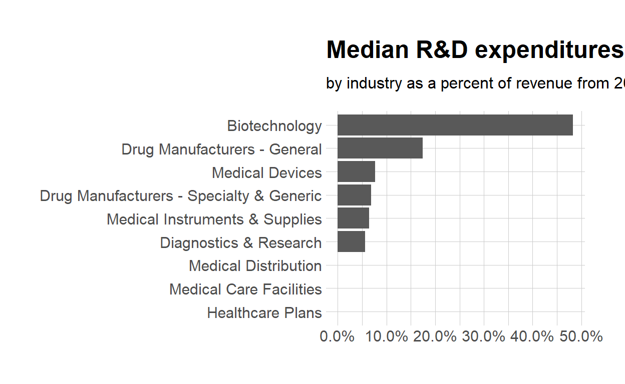
$ med_rnd_rev <dbl> 0.48317287, 0.05620271, 0.17451442, 0.0685187...- Create a static bar chart
use ggplot to initialize the chart
data is df
the variable industry is mapped to the x-axis reorder it based the value of med_rnd_rev
the variable med_rnd_rev is mapped to the y-axis
add a bar chart using geom_col
use scale_y_continuous to label the y-axis with percent
use coord_flip() to flip the coordinates
use labs to add title, subtitle and remove x and y-axes
use theme_ipsum() from the hrbrthemes package to improve the theme
ggplot(data = df,
       mapping = aes(
         x = reorder(industry, med_rnd_rev ),
         y = med_rnd_rev
         )) +
  geom_col() +
  scale_y_continuous(labels = scales::percent) +
  coord_flip() +
  labs(
    title = "Median R&D expenditures",
    subtitle = "by industry as a percent of revenue from 2011 to 2018",
    x = NULL, y = NULL) +
  theme_ipsum()
- Save the last plot to
preview.pngand add to the yaml chunk at the top
ggsave(filename = "preview.png",
       path = here::here("_posts", "2021-03-11-joining-data"))
- Create an interactive bar chart using the package
echarts4r
start with the data df
use arrange to reorder med_rnd_rev
use e_charts to initialize a chart the variable industry is mapped to the x-axis
add a bar chart using e_bar with the values of med_rnd_rev
use e_flip_coords() to flip the coordinates
usee_title to add the title and the subtitle
use e_legend to remove the legends
use e_x_axis to change format of labels on x-axis to percent
usee_y_axis to remove labels on y-axis-
use e_theme to change the theme. Find more themes here
df  %>%
  arrange(med_rnd_rev)  %>%
  e_charts(
    x = industry
    )  %>%
  e_bar(
    serie = med_rnd_rev,
    name = "median"
    )  %>%
  e_flip_coords()  %>%
  e_tooltip()  %>%
  e_title(
    text = "Median industry R&D expenditures",
    subtext = "by industry as a percent of revenue from 2011 to 2018",
    left = "center") %>%
  e_legend(FALSE) %>%
  e_x_axis(
    formatter = e_axis_formatter("percent", digits = 0)
    )  %>%
  e_y_axis(
    show = FALSE
  )  %>%
  e_theme("infographic")